In my last post, I showed you how to create a table of statistical tests using the command() option in the new and improved table command. In this post, I will show you how to gather information and create tables using the new collect suite of commands. Our goal is to fit three logistic regression models and create the table in the Adobe PDF document below.
Create the basic table
Let’s begin by typing webuse nhanes2l to open the NHANES dataset and then typing describe to examine some of the variables.
. webuse nhanes2l (Second National Health and Nutrition Examination Survey) . describe highbp age sex diabetes Variable Storage Display Value name type format label Variable label ------------------------------------------------------------------------------- highbp byte %8.0g * High blood pressure age byte %9.0g Age (years) sex byte %9.0g sex Sex diabetes byte %12.0g diabetes Diabetes status
The dataset includes age, sex, an indicator for high blood pressure (highbp), and an indicator for diabetes (diabetes).
A new strategy for building tables
We will fit three logistic regression models for the binary outcome highbp. For each model, we will use the logistic command to estimate the odds ratios and standard errors. Then we will use estat ic to estimate the Akaike’s information criterion (AIC) and Schwarz’s Bayesian information criterion (BIC) for each model. Our final table will include information for three models from six different commands.
Given the relative complexity of our table, we are going to use a new strategy to build it. We will use collect get to gather information from each command. Then we will use collect layout to define the layout of our table. Let’s do a simple example to illustrate this strategy before we begin the full table.
Let’s type collect get: before our first logistic regression command.
. collect get: logistic highbp c.age i.sex Logistic regression Number of obs = 10,351 LR chi2(2) = 1563.54 Prob > chi2 = 0.0000 Log likelihood = -6268.9975 Pseudo R2 = 0.1109 ------------------------------------------------------------------------------ highbp | Odds ratio Std. err. z P>|z| [95% conf. interval] -------------+---------------------------------------------------------------- age | 1.049042 .0013945 36.02 0.000 1.046313 1.051779 | sex | Female | .648767 .0280172 -10.02 0.000 .5961141 .7060706 _cons | .0887874 .0063561 -33.83 0.000 .0771641 .1021615 ------------------------------------------------------------------------------ Note: _cons estimates baseline odds.
Next let’s type collect layout to define the layout of a table with row dimension colname and column dimension result. I have used square brackets to include only the levels _r_b and _r_se from the dimension result. This will add columns for the coefficients and standard errors, respectively.
. collect layout (colname) (result[_r_b _r_se]) Collection: default Rows: colname Columns: result[_r_b _r_se] Table 1: 4 x 2 ------------------------------------ | Coefficient Std. error ------------+----------------------- Age (years) | 1.049042 .0013945 Male | 1 0 Female | .648767 .0280172 Intercept | .0887874 .0063561 ------------------------------------
That was easy! We created a basic table of regression output with two commands. The output tells us that collect get created a new collection named default.
Let’s repeat this strategy and add some options. Let’s begin by typing collect clear to clear any collections from Stata’s memory. Then let’s use collect create to create a new collection named MyModels.
collect clear collect create MyModels
Next let’s use the collect get option name() to gather the results from our logistic regression model in our collection named MyModels. Note that I have typed collect rather than collect get. The word “get” is not necessary.
collect, name(MyModels): logistic highbp c.age i.sex
I would also like to specify a new dimension and level for the results of my logistic regression model. I can do this using the tag() option. The basic syntax is tag(dimension[level]). The example below stores the results of the logistic regression model to the level (1) in the dimension model.
collect, name(MyModels) /// tag(model[(1)]) /// : logistic highbp c.age i.sex
The example above stores all the results from the model. But we will only need the coefficients and standard errors. We can specify a list of results to be automatically reported in the table by including those results after collect. The example below collects only the coefficients (_r_b) and the standard errors (_r_se) from the logistic regression model.
collect _r_b _r_se, /// name(MyModels) /// tag(model[(1)]) /// : logistic highbp c.age i.sex
Now we can use collect layout to create a table from the results we stored in level (1) of dimension model in the collection MyTables.
. collect layout (colname#result) (model[(1)]), name(MyModels) Collection: MyModels Rows: colname#result Columns: model[(1)] Table 1: 12 x 1 ------------------------ | (1) --------------+--------- Age (years) | Coefficient | 1.049042 Std. error | .0013945 Male | Coefficient | 1 Std. error | 0 Female | Coefficient | .648767 Std. error | .0280172 Intercept | Coefficient | .0887874 Std. error | .0063561 ------------------------
You may be wondering how I selected the row and column dimensions for collect layout. I could explain why this particular example worked. But it may not work for your tables. So let’s walk through the steps I used to figure it out.
Some details about collect layout
Let’s begin by typing collect dims to view a list of the dimensions in our collection.
. collect dims Collection dimensions Collection: MyModels ----------------------------------------- Dimension No. levels ----------------------------------------- Layout, style, header, label cmdset 1 coleq 1 colname 8 colname_remainder 1 model 1 program_class 1 result 43 result_type 3 rowname 1 sex 2 Style only border_block 4 cell_type 4 -----------------------------------------
The dimension result catches my eye because of the name and because it has 43 levels. We can view a list of the levels by typing collect levelsof result.
. collect levelsof result Collection: MyModels Dimension: result Levels: N N_cdf N_cds _r_b _r_ci _r_df _r_lb _r_p _r_se _r_ub _r_z chi2 chi2type cmd cmdline converged depvar df_m estat_cmd ic k k_dv k_eq k_eq_model ll ll_0 marginsnotok marginsok ml_method mns opt p predict properties r2_p rank rc rules technique title user vce which
The dimension result contains estimates of the coefficients, standard errors, and many other statistical results from our model. Let’s use collect layout to create a table for the dimension result.
. collect layout (result), name(MyModels) Collection: MyModels Rows: result Your layout specification does not uniquely match any items. Dimension colname might help uniquely match items.
That didn’t work. But the output suggests that including the dimension colname might help. The dimension named colname has eight levels and we can view a list of the levels by typing collect levelsof colname.
. collect levelsof colname Collection: MyModels Dimension: colname Levels: age 1.sex 2.sex c1 c2 c3 c4 _cons
The dimension colname includes the variable names, including factor variables, from our logistic regression model. It also contains levels named c1, c2, c3, and c4. Let’s add the row dimension colname and see what happens.
. collect layout (colname) (result), name(MyModels) Collection: MyModels Rows: colname Columns: result Table 1: 4 x 2 ------------------------------------ | Coefficient Std. error ------------+----------------------- Age (years) | 1.049042 .0013945 Male | 1 0 Female | .648767 .0280172 Intercept | .0887874 .0063561
That worked—we have a table! But the table raises an important question. The dimension result has 43 levels, and the dimension colname included levels like c1. Why aren’t all of those levels displayed in the table?
The answer is that collect layout only includes cells where there is a value associated with each level of both the row and the column dimensions. Recall that we requested that only the coefficients (_r_b) and standard errors (_r_se) from our model be displayed. And those coefficients and standard errors were only collected for the levels age, 1.sex, 2.sex, and _cons for the dimension colname.
Once we understand this concept, we can explore other layouts for our table. For example, we could stack the coefficients and standard errors under each variable in our model.
. collect layout (colname#result) (), name(MyModels) Collection: MyModels Rows: colname#result Table 1: 12 x 1 ------------------------ Age (years) | Coefficient | 1.049042 Std. error | .0013945 Male | Coefficient | 1 Std. error | 0 Female | Coefficient | .648767 Std. error | .0280172 Intercept | Coefficient | .0887874 Std. error | .0063561 ------------------------
We will eventually create a similar column of results for each of these three models. Recall that we created the dimension model with collect, tag(). Let’s view the levels of the dimension model by typing collect levelsof model.
. collect levelsof model Collection: MyModels Dimension: model Levels: (1)
For now, the dimension model has one level named (1), and we can specify model as our column dimension.
. collect layout (colname#result) (model[(1)]), name(MyModels) Collection: MyModels Rows: colname#result Columns: model[(1)] Table 1: 12 x 1 ------------------------ | (1) --------------+--------- Age (years) | Coefficient | 1.049042 Std. error | .0013945 Male | Coefficient | 1 Std. error | 0 Female | Coefficient | .648767 Std. error | .0280172 Intercept | Coefficient | .0887874 Std. error | .0063561 ------------------------
This approach to building tables in steps can be helpful if you are unsure how to begin. Start by typing collect dims to view the dimensions in the collection. Then use collect levelsof to view the levels of each dimension. Then experiment with collect layout to design your table. The output of collect layout will often provide helpful instructions.
Collecting results from multiple commands
Recall that we would also like to include the AIC and BIC for each model in our table, and we can estimate them by typing estat ic after we fit the model.
. estat ic Akaike's information criterion and Bayesian information criterion ----------------------------------------------------------------------------- Model | N ll(null) ll(model) df AIC BIC -------------+--------------------------------------------------------------- . | 10,351 -7050.765 -6268.998 3 12544 12565.73 ----------------------------------------------------------------------------- Note: BIC uses N = number of observations. See [R] BIC note.
The estimates of the AIC and BIC are stored in a matrix named r(S).
. return list matrices: r(S) : 1 x 6
And we can view the matrix by typing matlist r(S).
. matlist r(S) | N ll0 ll df AIC BIC -------------+------------------------------------------------------------------ . | 10351 -7050.765 -6268.998 3 12544 12565.73
We can refer to the AIC and BIC in the matrix r(S) using matrix subscripting. The general syntax to refer to an element in a matrix is matname[row,column]. Using this syntax, we can refer to the BIC as r(S)[1,6]. Column 6 is named BIC, so we can also refer to the BIC as r(S)[1,”BIC”].
. display r(S)[1,"BIC"] 12565.73
Let’s collect the AIC and BIC and store them in level (1) of dimension model in our MyModels collection.
collect AIC=r(S)[1,"AIC"] /// BIC=r(S)[1,"BIC"], /// name(MyModels) /// tag(model[(1)]) /// : estat ic
Then we can include them in our table by adding result[AIC BIC] to the row dimension of collect layout.
. collect layout (colname#result result[AIC BIC]) (model[(1)]), name(MyModels) Collection: MyModels Rows: colname#result result[AIC BIC] Columns: model[(1)] Table 1: 14 x 1 ------------------------ | (1) --------------+--------- Age (years) | Coefficient | 1.049042 Std. error | .0013945 Male | Coefficient | 1 Std. error | 0 Female | Coefficient | .648767 Std. error | .0280172 Intercept | Coefficient | .0887874 Std. error | .0063561 AIC | 12544 BIC | 12565.73 ------------------------
Notice that I did not include the “#” operator when I added the row dimension result[AIC BIC]. This is because AIC and BIC are not nested within each level of the dimension colname. I simply wanted to add rows for AIC and BIC at the bottom of the table.
Adding more models to the table
Let’s add a second model to our table. Notice that the commands below are nearly identical to the commands I used above. There are only two differences. First, I have used factor-variable notation to add the interaction of age and sex to the logistic regression model. And second, I am storing the results to level (2) of the dimension model.
collect _r_b _r_se, /// name(MyModels) /// tag(model[(2)]) /// : logistic highbp c.age##i.sex collect AIC=r(S)[1,"AIC"] /// BIC=r(S)[1,"BIC"], /// name(MyModels) /// tag(model[(2)]) /// : estat ic
We can use collect layout to make sure that it worked.
. collect layout (colname#result result[AIC BIC]) (model), name(MyModels) Collection: MyModels Rows: colname#result result[AIC BIC] Columns: model Table 1: 20 x 2 ---------------------------------------- | (1) (2) ---------------------+------------------ Age (years) | Coefficient | 1.049042 1.035184 Std. error | .0013945 .0018459 Male | Coefficient | 1 1 Std. error | 0 0 Female | Coefficient | .648767 .1556985 Std. error | .0280172 .0224504 Male # Age (years) | Coefficient | 1 Std. error | 0 Female # Age (years) | Coefficient | 1.028811 Std. error | .002794 Intercept | Coefficient | .0887874 .1690035 Std. error | .0063561 .0153794 AIC | 12544 12434.34 BIC | 12565.73 12463.32 ----------------------------------------
That worked, so let’s add a third model to our table. Let’s add the variable diabetes to our second model. And we will store the results to level (3) of the dimension model.
collect _r_b _r_se, /// name(MyModels) /// tag(model[(3)]) /// : logistic highbp c.age##i.sex i.diabetes collect AIC=r(S)[1,"AIC"] /// BIC=r(S)[1,"BIC"], /// name(MyModels) /// tag(model[(3)]) /// : estat ic
Let’s use collect layout again to make sure that it worked.
. collect layout (colname#result result[AIC BIC]) (model), name(MyModels) Collection: MyModels Rows: colname#result result[AIC BIC] Columns: model Table 1: 26 x 3 ------------------------------------------------- | (1) (2) (3) ---------------------+--------------------------- Age (years) | Coefficient | 1.049042 1.035184 1.034281 Std. error | .0013945 .0018459 .0018566 Male | Coefficient | 1 1 1 Std. error | 0 0 0 Female | Coefficient | .648767 .1556985 .1549363 Std. error | .0280172 .0224504 .0223461 Male # Age (years) | Coefficient | 1 1 Std. error | 0 0 Female # Age (years) | Coefficient | 1.028811 1.028856 Std. error | .002794 .0027958 Not diabetic | Coefficient | 1 Std. error | 0 Diabetic | Coefficient | 1.521011 Std. error | .154103 Intercept | Coefficient | .0887874 .1690035 .1730928 Std. error | .0063561 .0153794 .0157789 AIC | 12544 12434.34 12417.74 BIC | 12565.73 12463.32 12453.97 -------------------------------------------------
Now we have the basic layout of our table. All we need to do now is customize the layout and export it to an Adobe PDF document.
Use collect style to format the table
I will use collect style showbase, collect style row, collect style cell, and collect style header to customize the layout of our table. The commands in the code block below are the same commands I used in previous posts, so I won’t explain each step here. But I have included comments to refresh our memory.
// TURN OFF BASE LEVELS FOR FACTOR VARIABLES collect style showbase off // CHANGE THE INTERACTION DELIMITER collect style row stack, spacer delimiter(" x ") // REMOVE THE VERTICAL LINE collect style cell border_block, border(right, pattern(nil)) // FORMAT THE NUMBERS collect style cell, nformat(%5.2f) collect style cell result[AIC BIC], nformat(%8.0f) // PUT PARENTHESES AROUND THE STANDARD ERRORS collect style cell result[_r_se], sformat("(%s)") // LABEL AIC AND BIC collect style header result[AIC BIC], level(label)
Let’s type collect preview to check our work so far.
. collect preview ----------------------------------------- (1) (2) (3) ----------------------------------------- Age (years) Coefficient 1.05 1.04 1.03 Std. error (0.00) (0.00) (0.00) Female Coefficient 0.65 0.16 0.15 Std. error (0.03) (0.02) (0.02) Female x Age (years) Coefficient 1.03 1.03 Std. error (0.00) (0.00) Diabetic Coefficient 1.52 Std. error (0.15) Intercept Coefficient 0.09 0.17 0.17 Std. error (0.01) (0.02) (0.02) AIC 12544 12434 12418 BIC 12566 12463 12454 -----------------------------------------
Next I will use some options that are unique to this table. First, I will use the collect style cell option halign() to center the items and column headers in the table.
. collect style cell cell_type[item column-header], halign(center) . collect preview ----------------------------------------- (1) (2) (3) ----------------------------------------- Age (years) Coefficient 1.05 1.04 1.03 Std. error (0.00) (0.00) (0.00) Female Coefficient 0.65 0.16 0.15 Std. error (0.03) (0.02) (0.02) Female x Age (years) Coefficient 1.03 1.03 Std. error (0.00) (0.00) Diabetic Coefficient 1.52 Std. error (0.15) Intercept Coefficient 0.09 0.17 0.17 Std. error (0.01) (0.02) (0.02) AIC 12544 12434 12418 BIC 12566 12463 12454 -----------------------------------------
Then I will use the collect style header option level() to hide the labels for the row dimension result.
. collect style header result, level(hide) . collect preview ----------------------------------------- (1) (2) (3) ----------------------------------------- Age (years) 1.05 1.04 1.03 (0.00) (0.00) (0.00) Female 0.65 0.16 0.15 (0.03) (0.02) (0.02) Female x Age (years) 1.03 1.03 (0.00) (0.00) Diabetic 1.52 (0.15) Intercept 0.09 0.17 0.17 (0.01) (0.02) (0.02) AIC 12544 12434 12418 BIC 12566 12463 12454 -----------------------------------------
And finally, I will use the collect style column option extraspace to add an extra space between the columns. I think this makes it easier to read the table.
. collect style column, extraspace(1) . collect preview ---------------------------------------------- (1) (2) (3) ---------------------------------------------- Age (years) 1.05 1.04 1.03 (0.00) (0.00) (0.00) Female 0.65 0.16 0.15 (0.03) (0.02) (0.02) Female x Age (years) 1.03 1.03 (0.00) (0.00) Diabetic 1.52 (0.15) Intercept 0.09 0.17 0.17 (0.01) (0.02) (0.02) AIC 12544 12434 12418 BIC 12566 12463 12454 ----------------------------------------------
We did it! We collected the results from our models and customized the layout.
Export the table to an Adobe PDF document
I showed you how to export your tables to a Microsoft Word document in my previous posts. Let’s try something new and export our table to an Adobe PDF document. Most of the putpdf commands are identical to their corresponding putdocx commands, with the obvious exception that they begin with putpdf rather than putdocx. But there are a few important differences.
First, I have replaced putdocx paragraph, style() with putpdf paragraph, font() halign(). The first instance sets the font to a 26-point Calibri Light font and centers the text horizonally on the page. The second instance sets the font to a 14-point Calibri Light font and begins the text on the left of the page. The third instance does not specify a font() or halign() option, so the default 11-point Helvetica font is used.
Second, I have replaced the collect style putdocx option layout(autofitcontents) with the collect style putpdf options width() and indent(). The width(60%) option sets the width of the table to 60% of the full width of the page. The indent(1 in) option indents the table one inch from the left side of the page.
And third, I have used the note() option with collect style putpdf to add a note to the table to tell the reader that the table displays odds ratios with standard errors in parentheses.
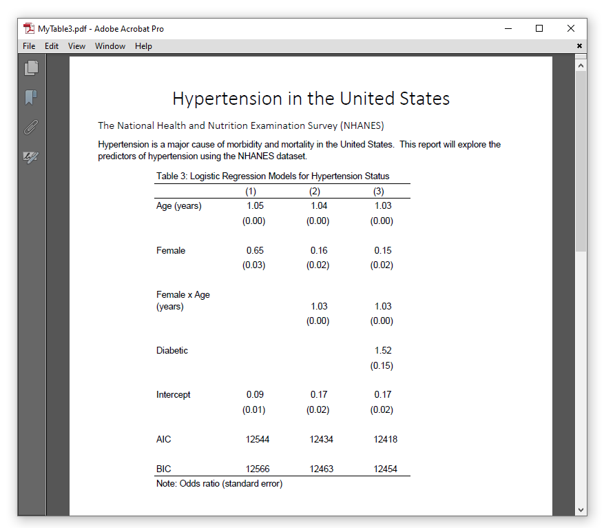
putpdf clear putpdf begin putpdf paragraph, font("Calibri Light",26) halign(center) putpdf text ("Hypertension in the United States") putpdf paragraph, font("Calibri Light",14) halign(left) putpdf text ("The National Health and Nutrition Examination Survey (NHANES)") putpdf paragraph putpdf text ("Hypertension is a major cause of morbidity and mortality in ") putpdf text ("the United States. This report will explore the predictors ") putpdf text ("of hypertension using the NHANES dataset.") collect style putpdf, width(60%) indent(1 in) /// title("Table 3: Logistic Regression Models for Hypertension Status") /// note("Note: Odds ratio (standard error)") putpdf collect putpdf save MyTable3.pdf, replace
The resulting Adobe PDF document looks like the image below.
In this post, we learned a new strategy to create tables using only the collect suite of commands. We used collect get to collect results from Stata commands, and we used collect layout to specify the layout of our table. We learned how to name our collections and store the results from commands to specific levels of dimensions.
You have probably noticed that we have used the same set of collect style commands in these blog posts. We could continue to copy and paste them into our future do-files, but there is an easier way to reuse collect style commands. In my next post, I will show you how to use collect style save and collect style use to save styles and reuse them with other tables. And I will show you how to use collect label save and collect label use to save labels for the levels of dimensions.